Lecture 25: PPO Demo Code
Proximal Policy Optimization (PPO) Demo
This code demonstrates the implementation of Proximal Policy Optimization (PPO), one of the most popular and effective policy gradient algorithms. PPO improves training stability by constraining policy updates to stay close to the previous policy.
Key concepts illustrated:
- Clipped surrogate objective function
- Generalized Advantage Estimation (GAE)
- Multiple epochs of minibatch updates
- Entropy regularization for exploration
- Old policy network for importance sampling ratio
The Ratio Clip: PPO’s Core Idea
In A2C, the actor loss is computed directly from the current log-probability of the sampled action:
\[L_\text{A2C} = -\, A_t \, \log \pi_\theta(a_t \mid s_t)\]This works, but it has a nasty failure mode: if a single mini-batch step pushes \(\pi_\theta\) far away from the policy that actually collected the data, the advantage estimates \(A_t\) stop being valid — they were computed for a different distribution. On-policy learning silently becomes off-policy, and training can diverge.
Importance sampling ratio
PPO addresses this by making the off-policy nature explicit. Let \(\pi_{\theta_\text{old}}\) be the policy snapshot that collected the trajectory, and \(\pi_\theta\) be the policy currently being optimized. The probability ratio
\[r_t(\theta) = \frac{\pi_\theta(a_t \mid s_t)}{\pi_{\theta_\text{old}}(a_t \mid s_t)}\]measures how much more (or less) likely the current policy is to pick action \(a_t\) compared to the policy that actually sampled it. At the start of the inner update loop, \(r_t = 1\) by construction. As gradient steps proceed, \(r_t\) drifts away from \(1\).
In code (see PPO.py:140):
ratio = (logprob - old_logprob[index]).exp()
The subtraction-in-log-space is the standard trick to avoid numerical blow-up when probabilities are tiny.
The unclipped surrogate
The naive “importance-sampled” policy-gradient objective is:
\[L^\text{IS}(\theta) = E_t \left[ r_t(\theta) \, A_t \right]\]This is correct in expectation as long as \(\pi_\theta\) stays close to \(\pi_{\theta_\text{old}}\). But it has no brakes: if some \(A_t\) is large and positive, the optimizer can push \(r_t\) arbitrarily high — the policy sprints toward that action and wrecks the trust region the advantage estimates were built on.
The clipped surrogate
PPO’s fix is a single line:
\[L^\text{CLIP}(\theta) = E_t \left[ \min\!\big( r_t \, A_t, \; \text{clip}(r_t, 1-\epsilon, 1+\epsilon) \, A_t \big) \right]\]with \(\epsilon \approx 0.2\). In code (see PPO.py:141-144):
surr1 = ratio * adv[index]
surr2 = ratio.clamp(1.0 - self._eps_clip, 1.0 + self._eps_clip) * adv[index]
act_loss = -torch.min(surr1, surr2).mean()
Why the min of two surrogates? Because the clip has to behave asymmetrically depending on the sign of the advantage:
| Case | \(A_t\) sign | What we want | What the clip does |
|---|---|---|---|
| Good action, already much more likely | \(A_t > 0\), \(r_t > 1+\epsilon\) | Stop climbing | clip caps \(r_t\) at \(1+\epsilon\); gradient is zero |
| Good action, still below old policy | \(A_t > 0\), \(r_t < 1\) | Keep climbing | Unclipped branch wins; normal gradient |
| Bad action, already much less likely | \(A_t < 0\), \(r_t < 1-\epsilon\) | Stop descending | clip floors \(r_t\) at \(1-\epsilon\); gradient is zero |
| Bad action, still above old policy | \(A_t < 0\), \(r_t > 1\) | Keep descending | Unclipped branch wins; normal gradient |
The min picks whichever surrogate is smaller (and therefore, after negation, whichever loss is larger) — this is the pessimistic bound. It says: “only trust the improvement I can guarantee inside the trust region; outside of it, don’t credit the policy for any further gain.”
The elegance is that there’s no KL constraint, no second-order optimization, no Lagrange multiplier — just a hard clamp and a min. The gradient automatically vanishes once \(r_t\) leaves the \([1-\epsilon, 1+\epsilon]\) band in the “wrong” direction, so the optimizer can safely run multiple epochs of mini-batch updates on the same rollout without blowing up the policy.
How PPO Differs from A2C (Lab 05)
PPO is best understood as “A2C with GAE, plus one extra safety mechanism.” Everything you built in Lab 05 — the Gaussian policy, the entropy bonus, the frozen-critic GAE, the two-optimizer setup — carries over verbatim. The only algorithmic addition is the ratio clip. Here is a side-by-side:
| A2C (Lab 05) | PPO (this demo) | |
|---|---|---|
| Actor loss | \(-A_t \log \pi_\theta(a_t \mid s_t)\) | \(-\min(r_t A_t, \text{clip}(r_t, 1\pm\epsilon) A_t)\) |
| Needs old policy snapshot? | No — actor is recomputed on the live net | Yes — old_act_net stores \(\pi_{\theta_\text{old}}\) for the ratio |
| Needs frozen critic snapshot? | Yes (old_v_net for GAE) |
Yes (same reason) |
| Safe to do many inner epochs? | Risky — policy drifts, advantages go stale | Yes — the clip caps per-step drift |
| Inner passes per rollout (typical) | 5 | 2–10; demo uses 2 outer × 1 inner per minibatch |
| Entropy bonus | Yes (\(\beta = 0.01\)) | Yes (\(\beta = 0.01\)) |
| Advantage estimator | GAE | GAE |
| Exploration mechanism | Stochastic Gaussian policy | Same |
What changes in the code? Compared to your Lab 05 A2C class, the PPO class adds exactly three things:
- A second target network,
old_act_net, created withcopy.deepcopyin the constructor and refreshed viaload_state_dictat the top of every outer iteration (PPO.py:170). It plays the same role for the actor thatold_v_netalready played for the critic. - A recomputation of the old log-probabilities under
torch.no_grad()at the start ofupdate()(PPO.py:98-102). These are treated as constants — they anchor the ratio. - The clipped surrogate loss replacing the plain policy-gradient loss (PPO.py:140-144).
Everything else — GAE recursion, entropy bonus, mini-batch loop, critic MSE loss, learning rates — is unchanged from Lab 05.
Result: A2C vs. PPO on Pendulum-v1
The figure below overlays training curves for the Lab 05 A2C implementation and the PPO demo, both with identical hyperparameters (\(\gamma = 0.95\), \(\lambda = 0.85\), entropy \(= 0.01\), actor lr \(= 10^{-4}\), critic lr \(= 10^{-3}\), mini-batch 32) on the same Pendulum-v1 environment.
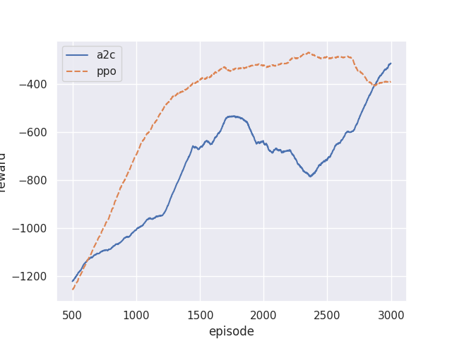
A few things to notice:
- Early learning is comparable. For the first few hundred episodes, both algorithms collect mostly random rollouts and the clip rarely activates — PPO behaves essentially like A2C.
- PPO reaches a higher asymptote with less variance. Once advantages start pointing in a consistent direction, PPO’s clipping prevents the aggressive mini-batch passes from over-shooting the trust region. A2C, lacking this brake, occasionally takes a mini-batch step that invalidates its own advantage estimates and the reward curve dips.
- PPO tolerates more inner passes. If you re-ran A2C with 10 inner passes instead of 5, you would see training destabilize; PPO’s clip means the same change is safe (and usually helpful, since you reuse each rollout more).
This is the core empirical case for PPO: same on-policy actor-critic recipe, one extra safety term, significantly more robust training.
# %%
import numpy as np
import gymnasium as gym
import torch
from torch import nn
from torch.distributions.normal import Normal
import torch.nn.functional as F

from tqdm.std import tqdm
import copy

device = 'cuda' if torch.cuda.is_available() else 'cpu'
# %%
env = gym.make('Pendulum-v1')
render_env = gym.make('Pendulum-v1', render_mode='human')
n_state = int(np.prod(env.observation_space.shape))
n_action = int(np.prod(env.action_space.shape))
print("# of state", n_state)
print("# of action", n_action)

# %%


def run_episode(env, policy):
    obs_list = []
    act_list = []
    reward_list = []
    next_obs_list = []
    done_list = []
    obs = env.reset()[0]
    while True:
        action = policy(obs)
        next_obs, reward, done, truncated, info = env.step(action)
        reward_list.append(reward), obs_list.append(obs), \
            done_list.append(done), act_list.append(action), \
            next_obs_list.append(next_obs)
        if done or truncated or len(obs_list) > 200:
            break
        obs = next_obs

    return obs_list, act_list, reward_list, next_obs_list, done_list

# %%


class PPO():
    def __init__(self, n_state, n_action):
        # Define network
        self.act_net = nn.Sequential(
            nn.Linear(n_state, 128),
            nn.ReLU(),
            nn.Linear(128, 128),
            nn.ReLU(),
            nn.Linear(128, 2*n_action),
        )
        self.act_net.to(device)
        self.old_act_net = copy.deepcopy(self.act_net)
        self.old_act_net.to(device)
        self.v_net = nn.Sequential(
            nn.Linear(n_state, 128),
            nn.ReLU(),
            nn.Linear(128, 128),
            nn.ReLU(),
            nn.Linear(128, 1),
        )
        self.v_net.to(device)
        self.v_optimizer = torch.optim.Adam(self.v_net.parameters(), lr=1e-3)
        self.act_optimizer = torch.optim.Adam(
            self.act_net.parameters(), lr=1e-4)
        self.old_v_net = copy.deepcopy(self.v_net)
        self.old_v_net.to(device)
        self.gamma = 0.95
        self.gae_lambda = 0.85
        self._eps_clip = 0.2
        self.act_lim = 2

    def __call__(self, state):
        with torch.no_grad():
            state = torch.FloatTensor(state).to(device)
            # calculate act prob
            output = self.act_net(state)
            mu = self.act_lim*torch.tanh(output[:n_action])
            var = torch.abs(output[n_action:])
            dist = Normal(mu, var)
            action = dist.sample()
            action = action.detach().cpu().numpy()
        return np.clip(action, -self.act_lim, self.act_lim)

    def update(self, data=None):
        obs, act, reward, next_obs, done = data
        obs = torch.FloatTensor(obs).to(device)
        next_obs = torch.FloatTensor(next_obs).to(device)
        act = torch.FloatTensor(act).to(device)
        with torch.no_grad():
            v_s = self.old_v_net(obs).detach().cpu().numpy().squeeze()
            v_s_ = self.old_v_net(next_obs).detach().cpu().numpy().squeeze()
            # calculate the pi_theta_k from current policy
            output = self.old_act_net(obs)
            mu = self.act_lim*torch.tanh(output[:, :n_action])
            var = torch.abs(output[:, n_action:])
            dist = Normal(mu, var)
            old_logprob = dist.log_prob(act)

        adv = np.zeros_like(reward)
        done = np.array(done, dtype=float)

        returns = np.zeros_like(reward)
        # # One-step
        # adv = reward + (1-done)*self.gamma*v_s_ - v_s
        # returns = adv + v_s
        # MC
        # s = 0
        # for i in reversed(range(len(returns))):
        #     s = s * self.gamma + reward[i]
        #     returns[i] = s
        # adv = returns - v_s
        # # GAE
        delta = reward + v_s_ * self.gamma - v_s
        m = (1.0 - done) * (self.gamma * self.gae_lambda)
        gae = 0.0
        for i in range(len(reward) - 1, -1, -1):
            gae = delta[i] + m[i] * gae
            adv[i] = gae
        returns = adv + v_s

        adv = torch.FloatTensor(adv).to(device)
        returns = torch.FloatTensor(returns).to(device)
        # Calculate loss
        batch_size = 32
        list = [j for j in range(len(obs))]
        for i in range(0, len(list), batch_size):
            index = list[i:i+batch_size]
            for _ in range(1):
                output = self.act_net(obs[index])
                mu = self.act_lim*torch.tanh(output[:, :n_action])
                var = torch.abs(output[:, n_action:])
                dist = Normal(mu, var)
                logprob = dist.log_prob(act[index])

                ratio = (logprob - old_logprob[index]).exp().float().squeeze()
                surr1 = ratio * adv[index]
                surr2 = ratio.clamp(1.0 - self._eps_clip, 1.0 +
                                    self._eps_clip) * adv[index]
                act_loss = -torch.min(surr1, surr2).mean()

                ent_loss = dist.entropy().mean()
                act_loss -= 0.01*ent_loss
                self.act_optimizer.zero_grad()
                act_loss.backward()
                self.act_optimizer.step()

            for _ in range(1):
                v_loss = F.mse_loss(self.v_net(
                    obs[index]).squeeze(), returns[index])
                self.v_optimizer.zero_grad()
                v_loss.backward()
                self.v_optimizer.step()

        return act_loss.item(), v_loss.item(), ent_loss.item()


# %%
loss_act_list, loss_v_list, loss_ent_list, reward_list = [], [], [], []
agent = PPO(n_state, n_action)
loss_act, loss_v = 0, 0
n_step = 0
for i in tqdm(range(3000)):
    data = run_episode(env, agent)
    agent.old_v_net.load_state_dict(agent.v_net.state_dict())
    agent.old_act_net.load_state_dict(agent.act_net.state_dict())
    for _ in range(2):
        loss_act, loss_v, loss_ent = agent.update(data)
    rew = sum(data[2])
    if i > 0 and i % 50 == 0:
        print("itr:({:>5d}) loss_act:{:>6.4f} loss_v:{:>6.4f} loss_ent:{:>6.4f} reward:{:>3.1f}".format(i, np.mean(
            loss_act_list[-50:]), np.mean(loss_v_list[-50:]),
            np.mean(loss_ent_list[-50:]), np.mean(reward_list[-50:])))
    if i > 0 and i % 500 == 0:
        run_episode(render_env, agent)

    loss_act_list.append(loss_act), loss_v_list.append(
        loss_v), loss_ent_list.append(loss_ent), reward_list.append(rew)

# %%
render_env.close()
scores = [sum(run_episode(env, agent)[2]) for _ in range(100)]
print("Final score:", np.mean(scores))

import pandas as pd
df = pd.DataFrame({'loss_v': loss_v_list,
                   'loss_act': loss_act_list,
                   'loss_ent': loss_ent_list,
                   'reward': reward_list})
df.to_csv("./ClassMaterials/Lecture_25_PPO/data/ppo.csv",
          index=False, header=True)