Lab 06: SAC
In this lab, you will implement Soft Actor-Critic (SAC) to solve Pendulum-v1.
Understand SAC
Read the OpenAI Spinning Up documentation on Soft Actor-Critic.
Focus on two ideas: the twin Q networks and entropy regularization. Feel free to skip the action-squashing (tanh) correction in the log-probability — we already clip actions explicitly as we did in PPO and DDPG.
Why SAC exists (context for this lab)
SAC is an off-policy actor–critic algorithm that combines three ingredients you have already seen separately:
- From DDPG (Lab 04): a replay buffer and target Q networks that let the agent learn from off-policy transitions.
- From A2C/PPO (Lab 05, Lecture 25): a stochastic Gaussian policy that explores by sampling, rather than by adding external noise to a deterministic policy.
- New in SAC:
- Twin Q networks — keep two independent critics and take the minimum of their estimates when building the TD target. This curbs the well-known overestimation bias of single-critic value learning (the same motivation as Double DQN / TD3).
- Maximum-entropy objective — the agent is trained to maximize \(\sum_t \big( r_t + \alpha\, H(\pi(\cdot \mid s_t)) \big)\) rather than just \(\sum_t r_t\). The extra entropy term, weighted by a temperature \(\alpha\), directly rewards the policy for staying stochastic, giving robust exploration without hand-tuned noise schedules.
Starter Code
Adapt code from DDPG (for the replay buffer and off-policy update) and PPO (for the stochastic Gaussian policy).
What to change
1. Stochastic policy
- Use the DDPG code as a base; port the stochastic actor from PPO.
- Keep the actor network structure similar to DDPG. Change only the last layer to output \(2 \cdot n_\text{action}\) values — the first half becomes \(\mu\), the second half becomes \(\sigma\). Remove the final
tanhon the raw output; applytanhonly to the \(\mu\) half (and scale byself.act_lim). The \(\sigma\) half must be made positive (e.g.abs()orsoftplus) and is often clamped to a small range such as[1e-3, 2]to avoid numerical blow-up. - Remove the target network for the actor (
target_act_net). SAC’s actor is trained directly against the current (live) Q networks, so no actor-target is needed — this matches the original paper.
2. Twin Q networks
- Rename the original
q_net→q1_netandtarget_q_net→target_q1_net. - Create a second Q network
q2_netwith the same architecture but independent initialization. (Usingcopy.deepcopy(self.q1_net)would give identical weights, which defeats the purpose of having two critics. Buildq2_netas a freshnn.Sequentialso it starts with different random weights. Only the target networks should be deep-copied from their live counterparts.)
self.q1_net = nn.Sequential(
    nn.Linear(n_state + n_action, 400),
    nn.ReLU(),
    nn.Linear(400, 300),
    nn.ReLU(),
    nn.Linear(300, 1)
)
self.q2_net = nn.Sequential(
    nn.Linear(n_state + n_action, 400),
    nn.ReLU(),
    nn.Linear(400, 300),
    nn.ReLU(),
    nn.Linear(300, 1)
)
self.q1_net.to(device)
self.target_q1_net = copy.deepcopy(self.q1_net)
self.target_q1_net.to(device)
self.q2_net.to(device)
self.target_q2_net = copy.deepcopy(self.q2_net)
self.target_q2_net.to(device)
- Give
q2_netits own Adam optimizer, just likeq1_net.
3. The soft Q target
SAC’s headline contribution is soft Q-learning: the TD target carries an extra entropy bonus so that the learned value function reflects both reward-to-go and expected future entropy.
Given a transition \((s, a, r, s', d)\) from the replay buffer, sample a next action \(\tilde{a}' \sim \pi_\theta(\cdot \mid s')\) from the current stochastic policy, then form:
\[y = r + \gamma\,(1 - d)\, \Big( \min_{i=1,2} Q_{\bar\phi_i}(s', \tilde{a}') \;-\; \alpha \, \log \pi_\theta(\tilde{a}' \mid s') \Big)\]The \(\min\) over the target critics controls overestimation; the \(-\alpha \log \pi\) term is the soft-Q entropy bonus. Note that the entropy term sits inside the \(\gamma(1-d)\) factor — at a terminal transition it drops out along with the bootstrap.
In code, computed inside torch.no_grad():
# Sample next action from the current policy at s'
output = self.act_net(next_obs)
mu = self.act_lim * torch.tanh(output[:, :n_action])
sigma = torch.abs(output[:, n_action:]).clamp(1e-3, 2)
dist = Normal(mu, sigma)
act_ = dist.sample()
logprob_ = dist.log_prob(act_).squeeze()

# Target Q values at (s', a')
q_input = torch.cat([next_obs, act_], axis=1)
q1_t = self.target_q1_net(q_input).squeeze()
q2_t = self.target_q2_net(q_input).squeeze()

# Soft-Q TD target
y = reward + self.gamma * (1 - done) * (torch.min(q1_t, q2_t) - self.alpha * logprob_)
Both q1_net and q2_net are then trained with MSE loss against the same target y.
self.alpha is the temperature: a hyper-parameter that trades off exploitation vs. exploration. Start with 0.2; you will vary it in the experiments below.
4. Reparameterization trick for the actor update
When training the actor, we want the gradient to flow through the sampled action back into \(\mu\) and \(\sigma\). A plain dist.sample() breaks this gradient (sampling is not differentiable). PyTorch provides the reparameterized sampler rsample(), which expresses the sample as \(a = \mu + \sigma \cdot \epsilon\) with \(\epsilon \sim \text{Normal}(0, 1)\) — this is differentiable in \(\mu\) and \(\sigma\).
dist = Normal(mu, sigma)
act_ = dist.rsample()              # differentiable sample
logprob_ = dist.log_prob(act_).squeeze()
The SAC actor loss is the negative of the soft Q value:
\[L_\text{act} = E_{s \sim D,\, \tilde{a} \sim \pi_\theta}\!\left[\, \alpha \, \log \pi_\theta(\tilde{a} \mid s) \;-\; \min_{i=1,2} Q_{\phi_i}(s, \tilde{a}) \,\right]\]i.e. the policy is pushed toward actions with high Q and high entropy (low \(\log \pi\)). This is almost the same as DDPG but with min-double-Q and the entropy term for the stochastic policy. In code:
q_input = torch.cat([obs, act_], axis=1)
q_min = torch.min(self.q1_net(q_input), self.q2_net(q_input)).squeeze()
loss_act = (self.alpha * logprob_ - q_min).mean()
Note that the Q networks here are the live ones (not targets) and we do not wrap this in no_grad — gradients need to flow through q_min → act_ → (mu, sigma) → act_net.
Write-up
- Run the program with three temperature settings:
self.alpha=0.0,0.2,0.5. Record the training log and plot the reward curves on the same axes. - Describe your observation of how
self.alphaaffects exploration and final return. What symptom do you see atalpha = 0.0? What symptom atalpha = 0.5? - Of SAC’s main contributions — twin Q networks, soft-Q learning / entropy bonus, and the reparameterized stochastic actor — which do you believe contributes most to the improvement over DDPG? Back your answer with an ablation or with a reasoned argument from the observed losses.
Deliverables and Rubrics
| Points | Requirement |
|---|---|
| 70 pts | PDF exported from the Jupyter notebook, including reward, loss_q, and loss_act curves and the final-score printout. |
| 15 pts | Performance: average reward reaches above −300 within 500 training episodes. |
| 15 pts | Reasonable answers to the write-up questions, supported by your experiment plots. |
Debugging Tips
If SAC performs worse than A2C:
- Check that both Q-networks are updating — print
loss_q1andloss_q2separately; they should evolve independently. - Verify the entropy term is in the Q target:
y = r + γ(1-d) * (min(Q1, Q2) − α · log π(ã′|s′)). - Ensure target networks are syncing correctly (either periodic hard copy or Polyak averaging — match your DDPG choice).
- Confirm the actor update uses
rsample(), notsample()— otherwise no gradient reaches the actor. - Make sure
q2_netis a freshly-initialized network, not adeepcopyofq1_net. Two identical critics collapse back to a single critic and you lose the overestimation fix. - If \(\sigma\) collapses to zero (policy becomes deterministic and reward stalls), check that you are clamping \(\sigma\) to a positive floor and that
alpha > 0.
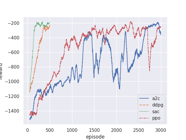
Reference training curves
Below are my training curves comparing SAC against DDPG and PPO on Pendulum-v1: