Lab 05: Advanced A2C
Goals
In this lab, you will extend the basic A2C algorithm to handle a harder continuous-control task, Pendulum-v1, by incorporating three ingredients that are essential for good on-policy learning:
- Continuous action support via a stochastic (Gaussian) policy.
- Entropy regularization to maintain exploration.
- Generalized Advantage Estimation (GAE) to reduce variance of the advantage signal.
Background
Why stochastic policies?
Unlike DDPG, which learns a deterministic policy \(\mu_\theta(s)\) and explores by adding external noise, A2C learns a stochastic policy \(\pi_\theta(a \mid s)\) that directly outputs a distribution over actions. Exploration is therefore built into the policy itself: each action is sampled from this distribution, and as the policy sharpens (variance shrinks), exploration naturally decays.
For continuous actions, a common choice is the diagonal Gaussian:
\[\pi_\theta(a \mid s) = \text{Normal}(\mu_\theta(s), \sigma_\theta(s))\]Both \(\mu\) and \(\sigma\) are produced by the same network head. This is why your actor network’s output layer has width 2 * n_action — half of the outputs are interpreted as means, the other half as (positive) standard deviations.
Why entropy regularization?
A stochastic policy can explore, but nothing in the vanilla policy-gradient objective stops it from collapsing prematurely into a near-deterministic policy (very small \(\sigma\)). Once that happens, the policy stops seeing alternative actions and gets stuck.
To counteract this, we add an entropy bonus to the loss:
\[L_\text{total} = L_\text{actor} - \beta \, \mathbb{E}\left[ H(\pi_\theta(\cdot \mid s)) \right]\]Maximizing entropy encourages the policy to keep spreading probability mass across actions. The coefficient \(\beta\) controls how strongly we insist on exploration — too large and the policy never commits to good actions, too small and it collapses. Noted that the \(L\) here is a loss that the optimizer minimizes, so we subtract the entropy bonus. Similarly, the \(L_\text{actor}\) is the negative of the policy gradient objective, which is the multiplication of the advantage and the gradient of the log probability.
Generalized Advantage Estimation (GAE)
The policy gradient relies on an advantage estimate \(A(s_t, a_t)\) that tells us how much better action \(a_t\) was than the “average” behavior of the current policy. Two natural choices sit at opposite ends of a bias–variance spectrum:
| Estimator | Formula | Bias | Variance |
|---|---|---|---|
| 1-step TD | \(\delta_t = r_t + \gamma V(s_{t+1}) - V(s_t)\) | High (depends on \(V\)) | Low |
| Monte Carlo | \(\sum_{l=0}^{\infty} \gamma^l r_{t+l} - V(s_t)\) | Low | High |
GAE gives you a single knob, \(\lambda \in [0, 1]\), to smoothly interpolate between them:
\[A_t^{\text{GAE}(\gamma, \lambda)} = \sum_{l=0}^{\infty} (\gamma \lambda)^l \, \delta_{t+l}\]which is computed very cheaply by a backward recursion over the episode:
\[A_t = \delta_t + \gamma \lambda \, A_{t+1}\]- \(\lambda = 0\) recovers the 1-step TD advantage (high bias, low variance).
- \(\lambda = 1\) recovers the Monte Carlo advantage (low bias, high variance).
GAE vs. Sarsa(λ): two sides of the same coin
You implemented Sarsa(λ) in Lab 02. It used eligibility traces to distribute a single TD error backward in time — credit for the TD error at step \(t\) was assigned to earlier state–action pairs with geometrically decaying weight \((\gamma\lambda)^k\). This is the forward–backward equivalence: you can either look forward (sum future TD errors) or look backward (maintain a trace of past visits), and both produce the same update in expectation.
GAE is the forward view of the same idea, applied to advantages instead of Q-value updates:
| Sarsa(λ) (Lab 02) | GAE (this lab) | |
|---|---|---|
| What does \(\lambda\) blend? | n-step Q-value backups | n-step advantage estimates |
| View | Backward (eligibility trace) | Forward (recursion over episode) |
| Used by | Tabular / function-approx TD control | Policy-gradient (actor–critic) |
| Updated object | \(Q(s,a)\) | Policy \(\pi_\theta\) via \(A_t\) |
| Bias–variance role of \(\lambda\) | Identical: λ=0 → bootstrap, λ=1 → MC | Identical: λ=0 → bootstrap, λ=1 → MC |
So when you tune gae_lambda, you are doing the same thing you did when tuning \(\lambda\) in Sarsa(λ) — choosing how aggressively to trust your critic’s current value estimate versus trust actual sampled returns. The mechanics look different (a backward recursion on the collected trajectory vs. an online trace), but the bias–variance knob is identical.
Why fix the critic while computing GAE?
GAE uses \(V(s_t)\) and \(V(s_{t+1})\) through the TD errors \(\delta_t\). If you computed advantages with the same v_net you are currently training, then every mini-batch step would shift \(V\) and therefore shift the target the actor is optimizing against — a moving target that destabilizes learning. The fix is identical in spirit to the target network in DQN/DDPG: snapshot the critic into an old_v_net at the start of the update phase, compute all advantages against that snapshot, and only then run multiple gradient steps.
Implementation
Your task is to extend the basic A2C code so it solves Pendulum-v1.
env = gym.make('Pendulum-v1')
Below is a summary of the key modifications you need to make. The reference network sizes and hyperparameters are collected at the bottom under Reference Hyperparameters.
1. Switch the actor to a Gaussian policy
Make the actor output both the mean and the standard deviation of a Normal distribution. A simple way is to have the final linear layer produce 2 * n_action outputs and split them:
- The first half becomes \(\mu\). Regulate it with
tanhand scale byself.act_limso it stays within the environment’s action range. - The second half becomes \(\sigma\). It must be positive — e.g., apply
abs()orsoftplus.
At action-selection time, build Normal(mu, sigma), sample an action, and (defensively) clip it to the valid range before passing it to the environment.
When computing the loss, recompute mu and sigma from the actor on the batched observations, form the same Normal distribution, and use dist.log_prob(act) to get \(\log \pi_\theta(a_t \mid s_t)\).
Type note: unlike DQN, actions are continuous-valued. Convert them with
FloatTensor, notLongTensor.
2. Add an entropy bonus to the actor loss
PyTorch’s Normal distribution gives you the entropy for free:
ent_loss = dist.entropy().mean()
Remember: we want entropy to be large, but the optimizer minimizes loss. Subtract a coefficient times the entropy from the actor loss:
act_loss = act_loss - 0.01 * ent_loss
A coefficient of 0.01 is a reasonable starting point. Too large, and the policy never commits; too small, and it collapses to a near-deterministic policy and stops exploring.
3. Compute advantages with GAE
After collecting one episode of (obs, act, reward, next_obs, done):
- Use a frozen snapshot of the critic (
old_v_net) to compute \(V(s_t)\) and \(V(s_{t+1})\) for every step. Do this undertorch.no_grad()and detach to numpy — these values are treated as constants during this update phase. - Compute the per-step TD error \(\delta_t = r_t + \gamma V(s_{t+1}) - V(s_t)\).
- Compute \(A_t\) by the backward recursion \(A_t = \delta_t + \gamma \lambda \, A_{t+1}\), walking from the last step to the first.
- Compute value targets as
returns = adv + v_sso the critic is trained toward \(V(s_t) + A_t\) (the λ-return). - Convert
advandreturnsto tensors on the device.
Set gae_lambda = 0.85 as your default.
Subtle point:
terminatedvs.truncated. Gymnasium’senv.step()returns five values:obs, reward, terminated, truncated, info. These two flags mean different things:
terminated = True→ the environment actually ended (e.g., the pole fell, the goal was reached). The episode’s future return really is zero, so you should bootstrap with \(V(s_{t+1}) = 0\).truncated = True→ the episode was cut off by a time limit (Pendulum-v1truncates at 200 steps). The state is not terminal — there would have been more reward to collect. You should still bootstrap from \(V(s_{t+1})\) as normal.Therefore, the
doneyou feed into your GAE mask (the(1 - done_t)factor) must beterminatedonly, notterminated or truncated. A common bug is to collapse both into a singledoneflag; onPendulum-v1that biases every episode’s final advantage downward because the 200-step cutoff is treated as if the pendulum had “really ended.” Usedone = terminated or truncatedonly to decide when to break out of the rollout loop.
Here is the reference function signature you should implement:
import numpy as np

def compute_gae(rewards, values, next_values, dones, gamma, lam):
    """Compute GAE advantages for a single trajectory.

    Args:
        rewards:     (T,) array of rewards r_t
        values:      (T,) array of V(s_t)
        next_values: (T,) array of V(s_{t+1})
        dones:       (T,) array, 1 if step t is terminal (else 0)
        gamma:       discount factor
        lam:         GAE lambda

    Returns:
        advantages: (T,) array of GAE advantages A_t
    """
    # delta_t = r_t + gamma * V(s_{t+1}) * (1 - done_t) - V(s_t)
    # A_t     = delta_t + gamma * lam * (1 - done_t) * A_{t+1}
    # (compute via a backward pass from t = T-1 down to t = 0)
    ...
Unit test for your GAE implementation
Copy-paste the block below after your compute_gae. It checks two cases you can verify by hand:
(1) the Monte-Carlo limit (\(\gamma = \lambda = 1\) with zero values), where \(A_t\) must equal the sum of future rewards, and
(2) a typical setting (\(\gamma = 0.99\), \(\lambda = 0.95\)) with explicit expected numbers.
import numpy as np

# Copy your compute_gae function here, then run these tests.

# --- Case 1: Monte-Carlo limit (gamma = lambda = 1, zero baseline).
# With V=0 everywhere, A_t must equal the sum of future rewards.
rewards     = np.array([1.0, 2.0, 3.0])
values      = np.array([0.0, 0.0, 0.0])
next_values = np.array([0.0, 0.0, 0.0])
dones       = np.array([0,   0,   1])
expected    = np.array([6.0, 5.0, 3.0])   # 1+2+3, 2+3, 3
adv = compute_gae(rewards, values, next_values, dones, gamma=1.0, lam=1.0)
assert np.allclose(adv, expected), f"Case 1 failed: got {adv}, expected {expected}"

# --- Case 2: gamma = 0.99, lambda = 0.95 on a 3-step terminal episode.
# Hand computation:
#   delta_0 = 1.0 + 0.99*0.5 - 0.5 = 0.995
#   delta_1 = 1.0 + 0.99*0.5 - 0.5 = 0.995
#   delta_2 = 1.0 + 0.99*0.0*(1-1) - 0.5 = 0.5
#   A_2 = 0.5
#   A_1 = 0.995 + 0.99*0.95*0.5       = 1.46525
#   A_0 = 0.995 + 0.99*0.95*1.46525   = 2.37306763
rewards     = np.array([1.0, 1.0, 1.0])
values      = np.array([0.5, 0.5, 0.5])
next_values = np.array([0.5, 0.5, 0.0])   # V(s_{t+1}) = 0 at the terminal transition
dones       = np.array([0,   0,   1])
expected    = np.array([2.37306763, 1.46525, 0.5])
adv = compute_gae(rewards, values, next_values, dones, gamma=0.99, lam=0.95)
assert np.allclose(adv, expected), f"Case 2 failed: got {adv}, expected {expected}"

print("All GAE tests passed!")
If either assertion trips, the most common bugs are: iterating forward instead of backward, forgetting the (1 - done_t) mask on the bootstrap term, or applying \(\gamma\lambda\) to \(\delta_t\) instead of to \(A_{t+1}\).
4. Snapshot the critic before the update phase
Before each update phase (i.e., each outer training iteration), copy the current v_net weights into old_v_net:
self.old_v_net.load_state_dict(self.v_net.state_dict())
old_v_net itself is created once, via copy.deepcopy(self.v_net), in the constructor. This is the direct analog of the DQN/DDPG target network — but because A2C is on-policy and updates each episode, we copy before every update rather than every N steps.
5. Use two optimizers and mini-batch over the episode
The actor and critic are trained with different loss functions, so give them separate Adam optimizers. A typical choice is:
- Actor:
lr = 1e-4 - Critic:
lr = 1e-3
The intuition for making the actor slower: the critic’s quality depends on whatever trajectories the current policy happens to collect. If the policy shifts aggressively on the back of a noisy critic, the two can destabilize each other. Keeping the actor conservative lets the critic catch up.
Within the update, split the collected episode into mini-batches of size ~32, and run several passes (e.g., 5) of actor and critic updates over those batches. This is the A2C analog of “gradient descent over the collected rollout.”
6. Put it together: the outer loop
At the top of every outer iteration:
- Run one episode with the current policy and collect
(obs, act, reward, next_obs, done). - Snapshot the critic into
old_v_net. - Call
update()several times on the same episode’s data. - Log
loss_act,loss_v,loss_ent, and the episode return.
Reference Hyperparameters
gamma = 0.95gae_lambda = 0.85- Entropy coefficient:
0.01 - Actor learning rate:
1e-4 - Critic learning rate:
1e-3 - Mini-batch size:
32 - Inner update passes per episode:
5
Here is the main training loop with these hyperparameters:
# %%
loss_act_list, loss_v_list, loss_ent_list, reward_list = [], [], [], []
agent = A2C(n_state, n_action)
loss_act, loss_v = 0, 0
n_step = 0
for i in tqdm(range(3000)):
    data = run_episode(env, agent)
    agent.old_v_net.load_state_dict(agent.v_net.state_dict())
    for _ in range(5):
        loss_act, loss_v, loss_ent = agent.update(data)
    rew = sum(data[2])
    if i > 0 and i % 50 == 0:
        print("itr:({:>5d}) loss_act:{:>6.4f} loss_v:{:>6.4f} loss_ent:{:>6.4f} reward:{:>3.1f}".format(i, np.mean(
            loss_act_list[-50:]), np.mean(loss_v_list[-50:]),
            np.mean(loss_ent_list[-50:]), np.mean(reward_list[-50:])))
    if i > 0 and i % 500 == 0:
        run_episode(render_env, agent)

    loss_act_list.append(loss_act), loss_v_list.append(
        loss_v), loss_ent_list.append(loss_ent), reward_list.append(rew)

# %%
render_env.close()
scores = [sum(run_episode(env, agent)[2]) for _ in range(100)]
print("Final score:", np.mean(scores))

import pandas as pd
df = pd.DataFrame({'loss_v': loss_v_list,
                   'loss_act': loss_act_list,
                   'loss_ent': loss_ent_list,
                   'reward': reward_list})
df.to_csv("./Lab_05_A2C_Advanced/data/a2c-gea.csv",
          index=False, header=True)
Comprehension Questions
Answer the following questions in your report. These are about understanding the algorithm, not your implementation.
Q1. When computing GAE, we use a frozen snapshot old_v_net rather than the live v_net. Describe, in concrete terms, what would go wrong if we recomputed advantages with the live v_net during the multi-pass inner update. (Hint: think about what the actor is optimizing against and whether that “target” stays fixed during the mini-batch loop.)
Q2. A2C and DDPG both solve continuous-control problems but handle exploration very differently. DDPG adds external Gaussian noise to a deterministic policy; A2C samples from a learned Gaussian and is regularized by an entropy bonus. Give one advantage and one disadvantage of A2C’s entropy-based exploration compared to DDPG’s external-noise exploration.
Q3. In the reference configuration, the actor’s learning rate (1e-4) is lower than the critic’s (1e-3). Explain why this asymmetry tends to stabilize training. What symptom would you expect to see in loss_v and in the reward curve if you swapped the two?
Experiment Questions
Back up your answers with plots.
-
Effect of
gae_lambda. Run training with three settings:0.7,0.85, and0.99. Plot all three reward curves on the same axes (moving-average smoothed) and describe the bias–variance trade-off you observe. Does any setting consistently win, or does it depend on the stage of training? -
Effect of the entropy coefficient. Run one additional experiment with the entropy coefficient set to
0(no entropy bonus) and one with it set to0.1(strong entropy bonus). What happens to the reward curve and to the variance of the policy over training? Connect your observation to the concept of premature policy collapse. -
(Open-ended) In your experiments, where do you see evidence that A2C’s gradients are noisier than DDPG’s? What practical consequences does this have for the number of episodes needed to solve
Pendulum-v1?
Deliverables and Rubrics
| Points | Requirement |
|---|---|
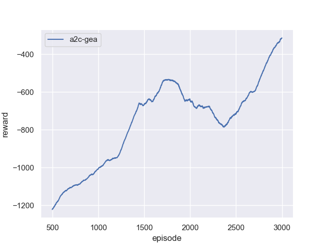
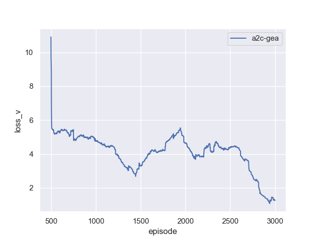
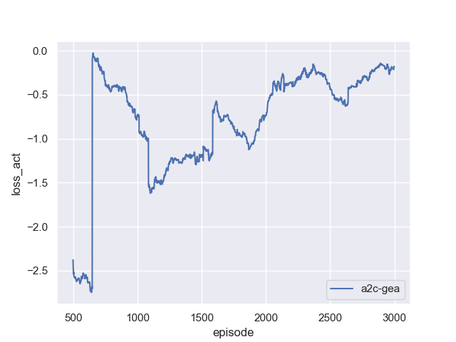
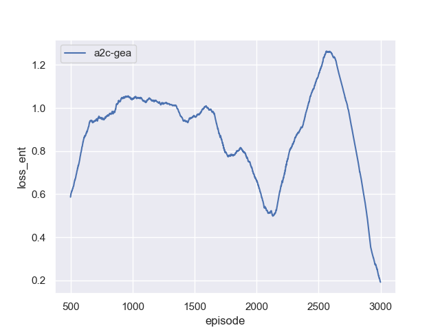
| 60 pts | PDF report (exported from Jupyter notebook) and Python source code. The report must include reward, loss_v, loss_act, and loss_ent curves over training. |
| 15 pts | Your implementation achieves a peak moving-average reward above −300. Partial credit: above −600 (some learning). Minimal credit: above −900. |
| 15 pts | The gae_lambda sweep experiment (0.7, 0.85, 0.99) with a comparative plot and written analysis of what you observe. |
| 10 pts | Reasonable answers to the comprehension and experiment questions above. |
Debugging Tips
-
Monitor all four signals.
loss_vshould stay bounded and trend downward (it is an MSE loss).loss_actis a policy-gradient loss — it is not meaningful as an absolute number, but sustained drift without reward improvement is a red flag.loss_entshould stay positive and slowly decrease as the policy sharpens; if it crashes to near-zero early, your policy has collapsed. -
If
loss_vexplodes into the thousands — first checkself.gamma. A large discount factor amplifies return variance. Dropping to0.95often fixes it. If it persists, you may be computing value targets via a long-horizon estimator; try loweringgae_lambda(closer to 1-step TD) to reduce variance in the target. -
If the policy collapses early (very low
loss_ent, stuck reward) — increase the entropy coefficient, or check that your \(\sigma\) output is not being driven to zero.abs()on the raw output can produce very small values; considersoftplusor adding a small floor. -
If actions cause environment errors — confirm you are clipping to
[-act_lim, act_lim]before callingenv.step().
Reference Training Curves