Starter Code

Check out my demo code on MC control below HERE

Implement Sarsa

1-Step Sarsa

With the demo code above, you should be able to quickly adapt the code to implement 1-step Sarsa. For the learning rate alpha, 0.01 is usually a good setting.

Note that you want to change the eps to 0 when testing and change back for training.

Different from the way to train MC, since TD method allows training on incomplete sequences, the training does not need to wait until one complete episode finishes. Therefore, the training iteration can be written as follows:

reward_list = []
n_episodes = 20000
for i in tqdm(range(n_episodes)):
    obs, _ = env.reset()
    while True:
        act = policy(obs)
        next_obs, reward, done, truncated, _ = env.step(act)
        next_act = policy(next_obs)
        policy.update(obs, act, reward, next_obs, next_act)
        if done or truncated:
            break

        obs = next_obs
    policy.eps = max(0.01, policy.eps - 1.0/n_episodes)
    mean_reward = np.mean([sum(run_episode(env, policy, False)[2])
                          for _ in range(2)])
    reward_list.append(mean_reward)

policy.eps = 0.0
scores = [sum(run_episode(env, policy, False)[2]) for _ in range(100)]
print("Final score: {:.2f}".format(np.mean(scores)))

import pandas as pd
df = pd.DataFrame({'reward': reward_list})
df.to_csv("./SomeFolderForThisLab/SARSA-1.csv",
          index=False, header=True)

Note that you need to change the file path SomeFolderForThisLab to match your setup.

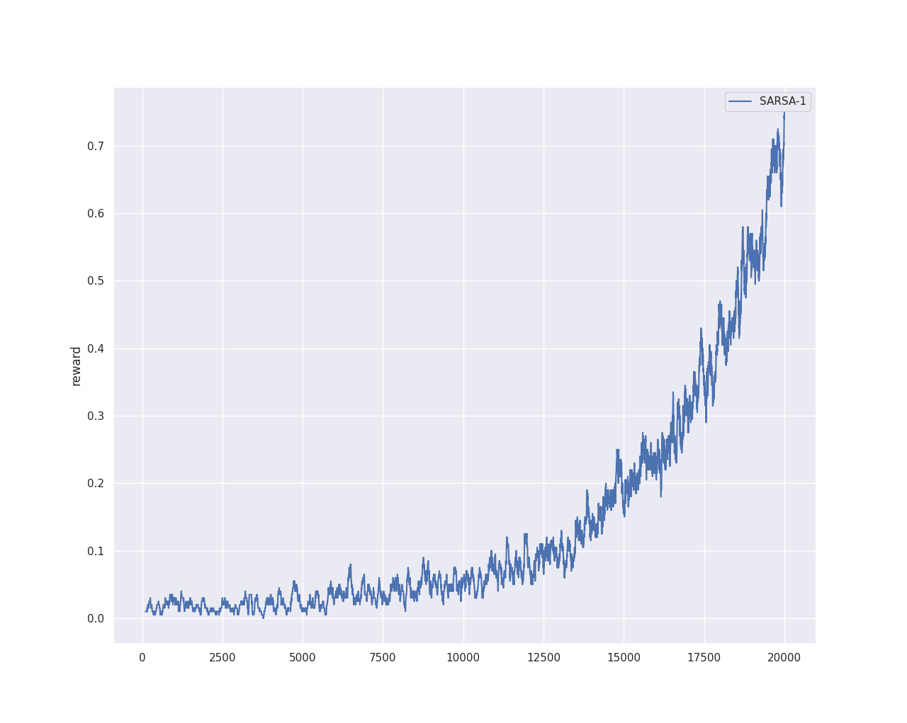
To show the training process, you can use the following command to plot the learning curve.

python ./SomeFolder/plot.py ./SomeFolderForThisLab reward -s 100

The plot.py is the script I provided in Lab Submission Guideline. If you need to download, here is the link again - plot.py. Note that the -s 100 means smoothing the curve(s) by running moving average over 100 data points. A sample output is shown below:

n-Step Sarsa

Change the code of 1-step Sarsa to implement:

• 2-step Sarsa
• 5-step Sarsa

Important: Make sure the cases of reward=1 are included into the calculation.

Similarly, save the testing results from each episode, and plot the learning curves from all Sarsa(s).

HINT: It is handy to use the double queue data type (deque) in Python. A quick tutorial can be found HERE.

Push it Further: Sarsa(λ)

To get full credit, I want you to implement Sarsa(λ) with eligibility traces. Study the online resources to understand how to implement it. Here is a good resource to start with: Sarsa(λ) Explanation. The material covers many advanced topics, but you only need to focus on the understanding and implementation of Sarsa(λ).

Draw the learning curve of Sarsa(λ) and compare it with the n-step Sarsa algorithms.

Write Report

Questions to answer in the report:

• (15 pts) Show the learning curves described above.
• (10 pts) Compare Sarsa algorithms with different steps, what are the pros and cons of n-step Sarsa with a large n.
• (5 pts) Compare Sarsa(λ) with n-step Sarsa, what are the pros and cons of using eligibility traces?

Deliverables and Rubrics

Overall, you need to complete the environment installation and be able to run the demo code. You need to submit:

• (70 pts) PDF (exported from jupyter notebook) and python code.
  • 1-step Sarsa 40 pts
  • n-step Sarsa 20 pts
  • Sarsa(λ) 10 pts
• (30 pts) Reasonable answers to the questions.