Lab Submission Guideline
1. Write your python code with interactive syntax
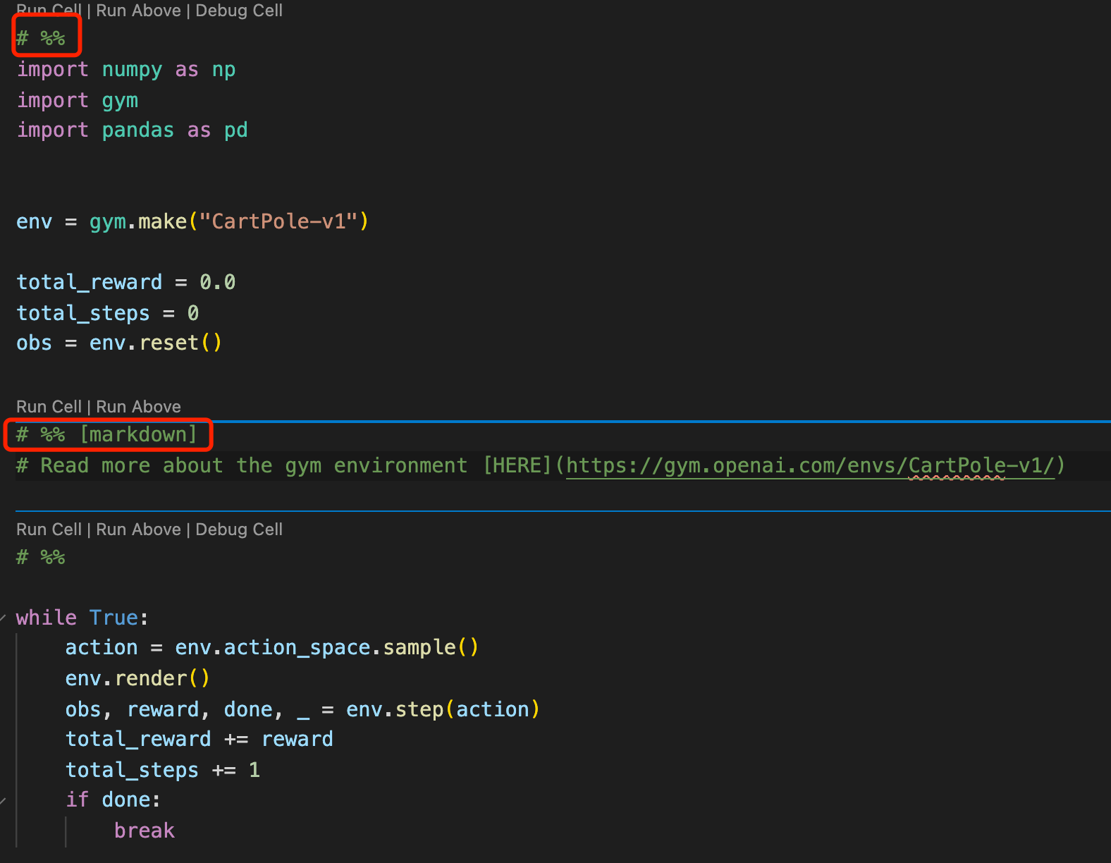
As shown above, use # %% to write python code and # %% [markdown] to write text content. To find out more markdown syntax, check the tutorial HERE.
2. Export the .py code as Jupyter Notebook .ipynb
Once you complete debugging your code, open the command console of vscode with shortcut CTR (or CMD on Mac) + SHIFT + P and type the command (usually you only need to type the first few words then you can see the option to select)
Jupyter: Export Current Python File as Jupyter Notebook
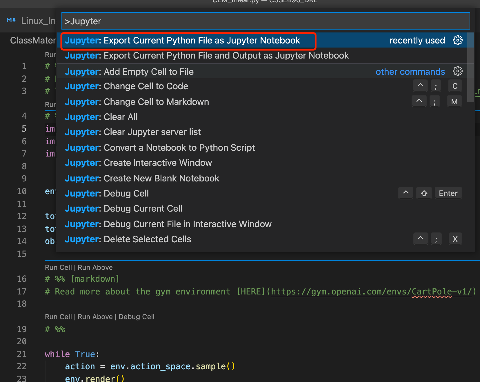
Select the export option to generate a Jupyter notebook file - .ipynb
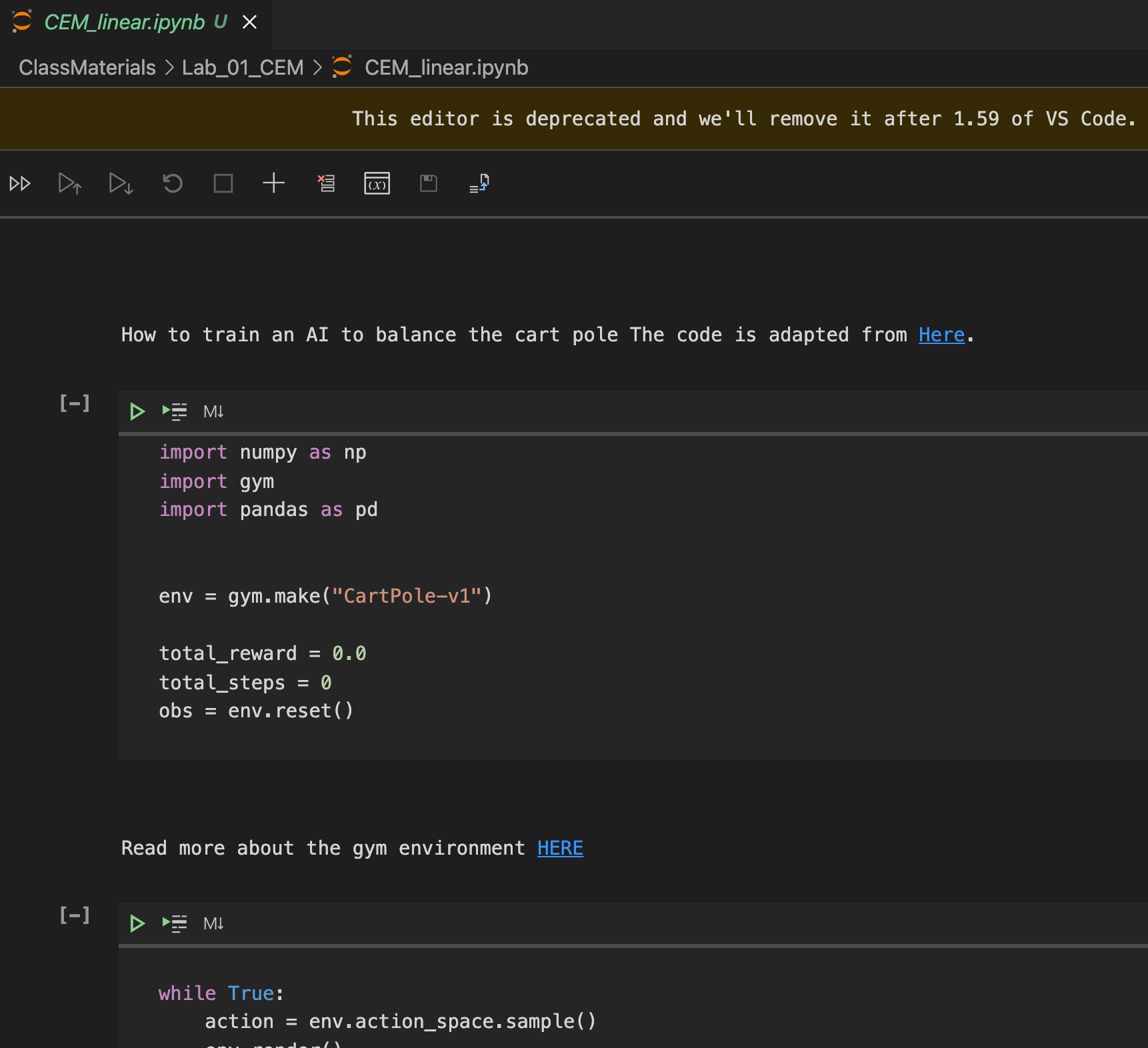
3. Run the .ipynb file to generate program output
Ideally, vscode will automatically open the .ipynb file with notebook editor where you can run and edit the code.
However, in case vscode doesn’t cooperate. Feel free to use the web-based Jupyter Notebook to open that file. The way to do this is go to your Linux command line, and activate your python virtual environment, then type
jupyter notebook
It will open Jupyter Notebook in the browser. You can follow the file path to open your .ipynb file.
Run your file in Notebook to generate program output.
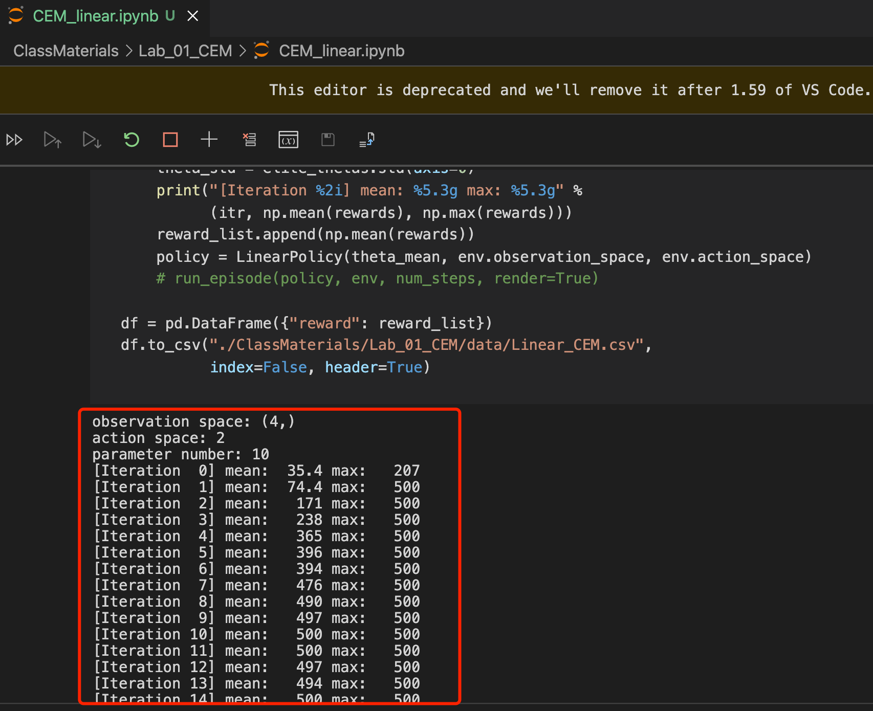
I will use the output as a reference to evaluate/judge if your program is correct. If needed, I will also run your .py to make sure the performance is “consistent”.
Don’t forget to save training log(s) to file:
In order to generate learning curve picture(s), you have to generate .csv file(s) in your program (usually at the end of your program). Don’t leave this part out in your .ipynb file.
4. Write report in .ipynb file including learning curve pictures
Plot result curves
Write python code (matplotlib or seaborn) to plot the results as figure(s). Here is a simple example code:
# %%

# Assuming you have saved rewards in the list reward_list
# Plot learning curve
plt.figure(figsize=(10, 6))
plt.plot(reward_list, linewidth=2)
plt.xlabel('Iteration', fontsize=12)
plt.ylabel('Average Reward', fontsize=12)
plt.title('CEM Learning Curve on CartPole-v1', fontsize=14, fontweight='bold')
plt.grid(True, alpha=0.3)
plt.tight_layout()
plt.show()

# Print statistics
print(f"Initial average reward: {reward_list[0]:.2f}")
print(f"Final average reward: {reward_list[-1]:.2f}")
print(f"Best average reward: {max(reward_list):.2f}")
print(f"Improvement: {reward_list[-1] - reward_list[0]:.2f}")
Alternatively, you can save the results into .csv files using code snippet like this,
import pandas as pd
df = pd.DataFrame({'reward': reward_list})
df.to_csv("./SomeFolderForThisLab/CEM_results.csv",
		  index=False, header=True)
Given the .csv files, you can use my plot script to generate learning curve pictures.
Download the plot.py file using the link above and use the command line to run the script. Here is an example of how to call the script:
If you have three .csv files named 1.csv, 2.csv and 3.csv under a folder with path ./data/, and each file includes three columns thing1, thing2, and thing3. To generate curves in column thing1 for all files, you can call the script like this:
python ./plot.py ./data/ thing1
This will plot the three curves of thing1 from all three files with different styles in one figure. This is very useful when you want to compare different methods in one figure.
Furthermore, to smooth (apply moving average) over the curve, you can add option -s 10 where 10 is the window size for moving average.
Save the picture: Once the figure is plotted, you can use the save button in the GUI to save the picture for later use.
Insert pictures into the report
Usually, I have specific questions for you to answer for each lab. To answers should all go to the Jupyter Notebook you’ve run. You need to create a new markdown cell to write the report.
For most cases if not all, I will require you to insert the learning curve picture into the report to demonstrate your result. To do this, you can use the markdown syntax for the image.

If you want to adjust the size of the picture, you can use the following html code
<img src="screen2.png" alt="screen2" style="zoom:40%;" />
Where src= is the file path of your picture and style="zoom:40%" is the place to adjust the size.
5. Export the .ipynb to PDF
After you finish writing the report in the Jupyter Notebook, run the complete code to generate results. Then
use export feature in both Jupyter extension in VSCode to export the notebook into PDF. You can do this
by clicking on the ... on the top bar of the notebook in VScode and select the export option then export the
notebook as a HTML file (Not the PDF option, because it requires xlatex, which we don’t need to install). Then find the HTML file in Windows File Explorer and open with your browser and print it as PDF.
6. To Submit
Go to the corresponding Moodle assignment page, and upload (drag and drop) the 1) PDF Report exported from .ipynb file and 2) the original py file.
For group submission: Each group only need to submit one copy of the files. Please put the names of group members on the top of the report.